Matrix Multiplicative Weights Update Method

A few days ago, I watched a lecture of Madhur Tulsiani on multiplicative weight update method and its applications to solving LPs. In this post, I am going to briefly describe about this. You can find the talk here.

Problem Statement

Consider a system of experts labelled 1,2,dots,N . There's a player who chooses an expert, say , and bears a loss equal to the loss of expert . The losses of each of the expert are revealed only after the player chooses the expert. This game continues on for, say, rounds. The losses of each expert will be different in different round. The player's strategy is to choose the experts in each round such that his total loss is minimized.

Example

As an example, let $l_i^{(t)}$ denote the loss associated with expert at time . We can have the following possible scenario:

Experts

Since the don't have complete information of the losses of each expert a prior, minimizing total loss makes little sense. Instead, we will try devising an algorithm where we perform as good as the best expert.

Greedy Algorithm

We will now prove that Greedy Algorithm can perform arbitrarily worse. Consider the following example:

Experts

wlog assume greedy algorithm picks the expert in following manner: Expert , Expert and so on. Clearly, this strategy accumulates a huge loss. The best strategy is to pick Expert at each stage.

MMW Algorithm

We will now describe the overall idea of MMW Algorithm:

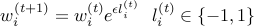
Maintain weights $w_i^{(t)} > 0$ .
Output distribution $(p_1^{(t)},p_2^{(t)},dots,p_N^{(t)})$ at every step. Note that $p_i^{(t)} propto w_i^{(t)}$ .
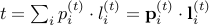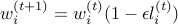
Loss at time $t = sum_i p_i^{(t)} cdot l_i^{(t)} = mathbf{p}_i^{(t)} cdot mathbf{l}_i^{(t)}$ .

The only remaining question is how to define $w_i^{(t)}$ and update them. There can be various possible approaches but the one we are going to use is based on Hedge Algorithm.

Hedge Algorithm

$w_i^{(t)} = 1 textup{~~} forall i$

$w_i^{(t+1)} = w_i^{(t)} e^{epsilon l_i^{(t)}} textup{~~} l_i^{(t)} in {-1,1}$

Analysis

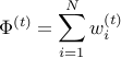
For the analysis of this function, we will define a potential function and compare the upper and lower bounds of loss.
The potential function is defined as:

$Phi^{(t)} = sum_{i=1}^N w_i^{(t)}$

Lower bound

$Phi^{(T+1)} ge exp(-epsilon sum_{t=1}^T l_i^{(t)}) textup{~~} forall i$

The above inequality follows from the fact that right hand quantity is $w_i^{(t+1)}$ and each of the $w_i^{(t)}$ 's is positive.

Upper bound

For the upper bound, we will be needing the following inequalities:

$forall x: textup{~} |x| le 1, textup{~~} e^x le 1+x+x^2$

$forall x, textup{~~} 1+x le e^x$

$Phi^{(T+1)} = sum_{i=1}^N w_i^{(T+1)} = sum_{i=1}^N w_i^{(T)} exp(-epsilon l_i^{(T)}) le sum_{i=1}^N w_i^{(T)} (1-epsilon l_i^{(T)}+epsilon^2) = sum_{i=1}^N w_i^{(T)} (1+epsilon^2) - epsilon sum_{i=1}^N w_i^{(T)} cdot l_i^{(T)}$

The second last line follows from using the above mentioned inequality and also the fact that $l_i^{(T)} in {-1,1}$ . Using the fact that 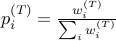$p_i^{(T)}=frac{w_i^{(T)}}{sum_i w_i^{(T)}}$ , we can write $Phi^{(T+1)}$ as

$Phi^{(T+1)} = (1+epsilon^2) Phi^{(T)} - epsilon (mathbf{p}^{(T)} cdot mathbf{l}^{(T)}) Phi^{(T)} = Phi^{(T)} (1 + epsilon^2 - epsilon mathbf{p}^{(T)} cdot mathbf{l}^{(T)}) le Phi^{(T)} exp (epsilon^2 - epsilon mathbf{p}^{(T)} cdot mathbf{l}^{(T)})$

Unfolding the $Phi^{T}$ , we obtain that

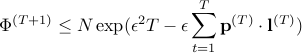
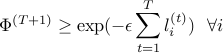
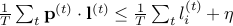
$Phi^{(T+1)} le N exp (epsilon^2 T - epsilon sum_{t=1}^Tmathbf{p}^{(T)} cdot mathbf{l}^{(T)})$

Using the two bounds obtained and taking log of both sides, we obtain,

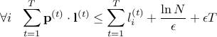
$forall i textup{~~} sum_{t=1}^T mathbf{p}^{(t)} cdot mathbf{l}^{(t)} le sum_{t=1}^T l_i^{(t)} + frac{ln N}{epsilon} + epsilon T$

The above inequality states that the loss incurred by our algorithm is worse off than the lost incurred by any expert (in particular, the best expert) by an additive factor which is independent of the expert's losses and depends only on the number of experts and rounds.

To view the above loss per round, divide the whole equation by .

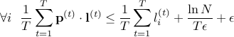
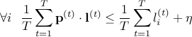
$forall i textup{~~} frac{1}{T} sum_{t=1}^T mathbf{p}^{(t)} cdot mathbf{l}^{(t)} le frac{1}{T} sum_{t=1}^T l_i^{(t)} + frac{ln N}{T epsilon} + epsilon$

Hence, as the number of rounds () increases, the algorithm performs better and the error drops. In fact, it can be shown that for $T ge frac{4 rho^2 ln n}{eta^2}$ ,

$forall i textup{~~} frac{1}{T} sum_{t=1}^T mathbf{p}^{(t)} cdot mathbf{l}^{(t)} le frac{1}{T} sum_{t=1}^T l_i^{(t)} + eta$

Exercises

A few exercises which can be tried out to fully internalize the concept:

Generalize for $l_i^{(t)} in [-1,1]$ .
What if $l_i^{(t)} in [-rho,rho]$ .
Using the update rule $w_i^{(t+1)} = w_i^{(t)} (1 - epsilon l_i^{(t)})$ and $l_i^{(t)} in [-1,1]$ , prove that $forall i, textup{~~} sum_{t=1}^T mathbf{p}^{(t)} cdot mathbf{l}^{(t)} le sum_{t=1}^T l_i^{(t)} + frac{ln N}{epsilon} + epsilon sum_{t=1}^T |l_i^{(t)}|$ .
Suppose $l_i^{(t)} in [0,rho]$ . Using the same update rule as above, prove that for $T ge frac{4 rho ln N}{eta^2}$ , $frac{1}{T} sum_t mathbf{p}^{(t)} cdot mathbf{l}^{(t)} le frac{1}{T} sum_t l_i^{(t)} + eta$ .